Thursday, November 16, 2023

Ratio boxes

I worked up a short new chapter for my Geometry book. It's about a device I'm calling ratio boxes, for want of a better word. When we have similar triangles, we have equal ratios of sides.

An example:

Above we have three similar right triangles, so we write down the sides in order from smallest to largest, and then repeat, going through each triangle in order.

The trick is that any four entries making a rectangle are a valid ratio from this data.

In particular, I'm hoping you may be able to see a quick proof of Pythagoras's Theorem.

There are several more examples. The most complicated is one from Inversive Transformation in a circle. The rule for the transformation is OA times OA' = r^2, where r is the radius of the circle with the solid line.

As we work through the example, you should be able to see how the ratio boxes dramatically simplify the bookkeeping involved in the proof. The chapter is on my Dropbox as a pdf.

The theorem is one of my very favorites.

Tuesday, November 7, 2023

Napoleon's Theorem

Napoleon's Theorem is a theorem some attribute (naturally enough) to Napoleon.

It says that if you take any triangle and draw equilateral triangles on each side, then the incenters of those triangles form a fourth equilateral triangle.

There is a variant in which the new triangles are drawn as reflections of the other ones, that is, inside the original triangle.

There is a terrific vector proof that I diagram here. (I think I got the idea for the proof from Alexander Bogomolny, but I can't find it at the moment. Wonderful site).

Define vectors for paths to and from the incenters based on the following.
Then apply a simple test for the adjacent sides of an equilateral triangle:
The details depend on the definition of the direction of rotation, and the path taken around the putative equilateral triangle. Details in the links below. Here is a variant of the problem:
My write-up is here. Probably the neatest thing is we get the variant basically for free, once the setup is done. I also (finally) got a proof on ProofWiki here as well as the variant (here)

Friday, September 1, 2023

Newton's series for the exponential

I've been reading the first chapter of Dunham's Calculus Gallery again (available here).

It starts with a discussion of Newton realizing that the binomial theorem (a+b)^n also applies for rational r as in (a+b)^r. In that case, the series does not terminate but is infinite. There is a deep discussion of how he came to that by Dennis and Addington, here.

Many great things come out of that including series for the logarithm and inverse sine and several series for π. Dunham also illustrates how Newton inverted or reversed series, for example to turn the inverse sine into the sine and the logarithm into the exponential.

I have new write-ups posted on github including an introduction to the standard binomial (pdf), as well as a second one working through the examples of of Dunham's chapter (pdf), including the process of inverting series, and a derivation of the exponential, as Newton did it.

Dunham left that to the reader. I haven't been this excited since Gil Strang led me to the integral that Newton solved, showing that for an inverse square force the mass acts as a point mass. To see it through Newton's eyes is a rare treat.

I found versions of Newton's manuscripts online (some in Latin), but haven't yet located the material on the binomial and on series.

I know I would have been very excited to find my second chapter linked here. Since visitors here have dropped from thousands to double digits, one can only hope that someone will click through and be excited as well.

Many thanks to a reader on math.stackexchange for pointing out my elementary error in a nice way, which allowed me to finish the last bit.

Monday, August 7, 2023

Archimedes and the Broken chord

The theorem of the "broken chord" is ascribed to Archimedes, although his original work has been lost. It was analyzed by the Arabic mathematician Al-Biruni in his Book on the Derivation of Chords in a Circle.

[UPDATE: I have made a translation and commentary of a German translation of this book. It is here. ]

Here is the general setup:

Let A and C be any two points on a circle. Let M be equidistant from both so that arc AM is equal to arc MC. Let B be another point on the circle, lying between A and M, so that AB < BC.

Drop the perpendicular from M to F on BC.

We claim that AB + BF = FC.

I will not spoil the fun by giving the proofs here. But these are eight constructions I know about.

Draw E such that AB = EC. (As an alternative approach, draw E such that BF = FE).

Draw the rectangle such that H is on the circle.
Extend BC such that DF = FC.
Draw E such that BF = FE and D such that BM = MD.
Draw E such that BF = FE and extend ME to G.
Extend BC and MF and draw DAG colinear.
At this point, I discovered a German translation of al Biruni's book (by Suter, link below). Therefore, I switched notation to match his figures. I can select the text in Preview, then Google Translate does a good job with it.

Extend BG as shown.

Extend the perpendicular DE as shown. Draw AG. Draw the diameter DK. (Hint: DK is perpendicular to AG).
Sources: Drakaki, al Biruni, Suter. There is a chapter in my geometry book on this. The chapter as a pdf is here, and the github repo for the book is here.

Thursday, June 22, 2023

Killing geometry

I think it's fair to say that math is not my granddaughter's favorite subject. The whole debate about whether some people are inherently good at math and some are not, is for another day. It is probably relevant that she is using online materials to learn.

I've been excited because she's starting geometry, and I really like the subject. So I am presented with this (I'm reconstructing) as the first problem.

There are so many things wrong with this that it's hard to know where to start. The biggest one is that she has not previously seen a problem like this being solved. The idea seems to be that students learn best when they figure everything out for themselves. Naturally, she's lost.

The second major issue is that whoever designed this curriculum thinks that in studying geometry, the student should spend most of the time practicing the skills from previous years. Hence the injection of algebra and arithmetic into this problem, where it really does not belong.

Beyond that, there is a misplaced emphasis on exact calculation, as if the measure of angles is the heart of the subject.

And there is a pedantic distinction between the name of an angle and its measure. Granted, this is a distinction worth being made, but then, move on. There is no harm and great simplification in using the name to refer to both things.

This creeps into the discussion in other ways. In the next problem, the phrase linear pair is insisted upon, as if distinguishing the case where two angles add up to two right angles (I mean, 180°) really matters. It's that misplaced emphasis on calculation again.

They insist on using the classical notation invented by the Greeks. As everyone knows, it's confusing to constantly refer back to a diagram and then say, now was that angle ABC or CBD? It is so much better to use θ and φ, or even, gasp, s and t. Having the right notation frees the mind to think about what's important.

The geometry content of this question can be reduced to restating the definition: to bisect an angle means to cut it in half. The two resulting parts have equal measure. Even better, show how the construction can be done, and then, have a discussion about why it works.

Now, that's worth talking about.

Tuesday, June 20, 2023

Acheson's Geometry

One of my favorite books is David Acheson's The Wonder Book of Geometry (Amazon here).

I especially enjoyed the proof that similar right triangles have equal ratios of sides. Here is how I might expand it in a slightly.

Draw a rectangle and then add one of the diagonals.

This forms two right triangles which are congruent (by SSS or SAS).

Any rectangle is divided by its diagonal into equal areas above and below the line.

Next, introduce a point on the diagonal and draw two lines, one vertical and one horizontal. This forms more rectangles. Divide each of them along their diagonals (which lie along the original one).

All six triangles in the figure are similar, having all three angles equal. (Prove this using some combination of vertical and complementary angles and the alternate interior angles theorem).

As before, the two triangles shaded blue have equal area, as do the two shaded red.

The key step is to realize that since the whole area above the diagonal in the original rectangle is equal to that below, light blue is equal to dark blue, and light red is equal to dark red, the remaining areas are also equal.

tall skinny rect + light blue + light red = short fat rect + red + blue.

Coloring one of those sub-rectangles for clarity, we have shown (in other words) that white is equal to gray in the figure below.

The area in white is Ab and that in gray is aB. Equate them to obtain Ab = aB, and then divide, giving A/a = B/b.

Also, since A/a + 1 = (A + a)/a = B/b + 1 = (B + b)/b, either of the smaller triangles has the same ratios as the big ones that span the entire original rectangle.

Here is his figure:

From there, it is not too difficult to derive the Pythagorean theorem.

Except that first we need the converse theorem, which seems a bit tricky.

However, playing with the ratio above, we see that if Ab = aB, then not only A/a = B/b but also A/B = a/b.

Let A/a = k = B/b. Then we have that A = ka, and B = kb.

Place two right triangles with equal ratios of sides next to each other, and grow the small one by a factor of k by extending the base, preserving the acute angle at the base. Say we set the new length of the base to be ka.

Then, by the forward theorem we still have equal ratios, meaning that the height is equal to kb, which as we saw is equal to B. Therefore the top vertices superimpose at the same point.

Therefore, the two triangles are congruent, and equality of angles follows. Since we maintain equality of two of three angles in growing the triangle, we preserve all three.

Here is a proof without words for the Pythagorean theorem, growing triangles in the same fashion:

By a simple extension, the general result can be proved, all angles equal means equal ratios of sides, for any triangle.

Update: I realize now that the last two examples depend on extending the equal ratios result to the hypotenuse of the similar right triangles. Of course, one can use the Pythagorean theorem and do some algebra with k^2. (Relying on Euclid's famous I.47 which uses SAS).

Alternatively, here's a nice simple proof. In any right triangle, drop the altitude to the hypotenuse, h. This forms two more similar triangles.

Form the ratio of the longer side (not the hypotenuse) to the shorter side in each of the three similar triangles: h/x = y/h = b/a. But b/a is also the ratio of the hypotenuse when comparing the medium and small triangles, and the equality says that this ratio is the same as h/x the ratio of the short sides comparing the same triangles. This completes the proof.

Monday, June 19, 2023

Exploring Hawaii

Continuing from the previous post, I thought I would summarize how to drill down to individual polygons in a GeoDataFrame containing the Hawaii data.

I put the code to load the data in another file and imported it, so we start with hw.gdf.

gdf = hw.gdf       # gdf is a GeoDataFrame
print(gdf.shape)   # (1,6) a single row
gs = gdf.geometry  # gs is a GeoSeries

So gdf.geometry (or gdf['geometry'], it's basically the same) is a GeoSeries object containing all the geometry data of the original data frame. The GeoSeries allows indexing by the special .iloc notation (below). The first item is a MultiPolygon, a collection of Polygon objects. These are obtained from the Multipolygon with the geoms attribute.

mp = gs.iloc[0]    # mp is a MultiPolygon
p0 = mp.geoms[0]   # p1 is a Polygon
ext = p0.exterior  # ext is a LinearRing

We want to do some shapely geometry operations with the LinearRing. The reason to do all this is that there doesn't seem to be anything in the data identifying the individual islands. The rest of the listing (below) shows the code.

The last step is to plot the data, and this is best done with the original GeoDataFrame's plot method. It is key to capture the returned Axes to use for adding text later.

The task of actually annotating the plot is fussy and i direct you to the github repo for that.

The code below prints:

> p3 explore_hawaii.py
(1, 6)
(9, 6)
0 Hawaii
2 Ni'ihau
3 Kauai
4 Molokai
5 Kaho'olawe
6 Maui
7 Lanai
8 O'ahu
8 Ford Island
> 

We now have assigned names for each of the Polygons representing islands. Ford Island (poly no. 1) does not seem to "contain" the point I picked for it, but that point is contained in the polygon for O'ahu.

import sys,os,subprocess
import geopandas as gpd

import matplotlib as mpl
import matplotlib.pyplot as plt
from shapely.geometry import Point

import hawaii as hw

#---------------------------------

fig,ax = plt.subplots()

gdf = hw.gdf        # gdf is a GeoDataFrame
print(gdf.shape)   # (1,6) a single row
gs = gdf.geometry  # gs is a GeoSeries

mp = gs.iloc[0]    # mp is a MultiPolygon
p1 = mp.geoms[0]   # p1 is a Polygon
ext = p1.exterior  # ext is a LinearRing

# this plots all the islands the same color
# gdf.boundary.plot(ax=ax,cmap='magma')

# so dissolve the Multi collection
exp = gdf.explode(index_parts=True)
print(exp.shape)   # (9,6) 9 islands

# we want to know which island is in each row
# a random point inside p1 (island of Hawaii)

D = {"Hawaii":[-155.519783,19.625055], 
     "Kaho'olawe":[-156.607857,20.550829],
     "Kauai":[-159.567160,22.017814],
     "Lanai":[-156.930387,20.834303],
     "Maui":[-156.279557,20.758340],
     "Molokai":[-156.986996,21.134644],
     "Ni'ihau":[-160.148047,21.904692],
     "O'ahu":[-157.968125,21.488976],
     "Ford Island":[-157.959627,21.363596]}

# each row of exp is a Series (not a Polygon)
def f(row):
    poly = row.geometry
    n = row.name[1]
    for k in D:
        xy = D[k]
        if poly.contains(Point(xy)):
            print(n,k)
        
exp.apply(f,axis=1)

Sunday, June 18, 2023

Geopandas and maps

Recently I've been exploring maps again, using GeoPandas in Python. I found it confusing at first, but that was mainly because I didn't understand the underlying technology very well, especially Pandas and the shapely geometry library. I've had to brush up on matplotlib, as well.

The figure above plots three thrips that we took to the US southwest, with a focus on the canyon country and Colorado. They were great trips, on highways and off the interstate. I wanted to memorialize them to help me remember. Of course Google Maps is pretty good for this stuff. Here is a route from LA-SLC-SF. I drove these legs many times in my youth.

But I wanted more control.

I use Homebrew to obtain my own Python3, rather than relying on Apple's build that is provided with macOS. Some people dislike Homebrew, but I'm not one of them. I never have any trouble with my (simple) "stack", and if I did, I would just use a virtual environment.

One thing that has changed over time is the need to use sudo to install Homebrew, which is moderately annoying, but I believe that happened because macOS now insists that /usr/local be owned by root. Perhaps I should put Homebrew in a different location, but I haven't.

In any case, I get the necessary packages by

python3 -m pip install --upgrade pip
python3 -m pip install -U numpy
python3 -m pip install -U pandas
python3 -m pip install -U matplotlib
python3 -m pip install -U geopandas

Then, all you need is some data. The main download page for the US Census is here. But the file I'm actually using for the boundaries of US states is at the bottom of this directory: gz_2010_us_040_00_5m.zip. Normally, geopandas should be able to read a ZIP file directly, but this one, you must unzip (or at least, that's what I did). Then

>>> import geopandas as gpd
>>> fn = 'gz_2010_us_040_00_5m'
>>> gdf = gpd.read_file(fn)
>>> gdf
         GEO_ID  ...                                           geometry
0   0400000US01  ...  MULTIPOLYGON (((-88.12466 30.28364, -88.08681 ...
..
[52 rows x 6 columns]
>>> gdf.columns
Index(['GEO_ID', 'STATE', 'NAME', 'LSAD', 'CENSUSAREA', 'geometry'], dtype='object')
>>>

It's as simple as that! To follow what I did, take a look at the github repo for this project.

A few quick tips. First, GeoPandas does things the Pandas way. So to get all the data for the state of Hawaii, say, you do:

sub = gdf[gdf['NAME'] == 'Hawaii']

or even

sub = gdf[gdf['STATE'] == '15']

where NAME and STATE are columns of the dataframe (and the FIPS code for Hawaii is 15). I think of an expression like that as a selector.

sel = gdf['NAME'] == 'Hawaii'

but it is actually a pandas "Series" of boolean values which the GeoDataFrame accepts as input for the indexing operator. The rules for what pandas will accept as a selector are much stricter than I would like. However, I discovered that a simple Python list of booleans will also work.

>>> def f(e):
...     if e.endswith('ii'):
...         return True
...     return False
... 
>>>
>>> sel = [f(e) for e in gdf['NAME']]
>>> gdf[sel]
         GEO_ID  ...                                           geometry
11  0400000US15  ...  MULTIPOLYGON (((-155.77823 20.24574, -155.7727...

[1 rows x 6 columns]
>>> 

Note that the original index is retained. It can also be useful to get a sense of what is in a column by doing
>>> L = list(gdf['LSAD'])
>>> L
[nan, nan ..]
>>> list(set(L))
[nan, nan ..]
>>>

but not in this case. Also, I notice that the old trick set(L) doesn't work with nan (not a number). Which is weird, because I would have thought it was from numpy
>>> import numpy as np
>>> L = [np.nan,np.nan]
>>> set(L)
{nan}
>>> list(set(L))
[nan]
>>>

It's important to realize how shapely.geometry objects are structured, at least, if what you want to do is get your hands on the underlying data. You can see that we have a MULTIPOLYGON but it is frustrating to get at it.

>>> sub = gdf[sel]
>>> sub
         GEO_ID  ...                                           geometry
11  0400000US15  ...  MULTIPOLYGON (((-155.77823 20.24574, -155.7727...

[1 rows x 6 columns]
>>>

The first thing is that the result of sub['geometry'] (or sub.geometry) is a geopandas.geoseries.GeoSeries object and it can be subscripted. Not in the usual way but by
>>> mp = sub['geometry'].iloc[0]

I used mp for MULTIPOLYGON. That guy has component geoms, in fact, 9 of them. We can get the first one by
>>> poly = mp.geoms[0]

This will turn out to be the Big Island, Hawai'i. Any polygon has an exterior (and an optional interior, i.e. a hole). The exterior has coords which have an attribute xy so we do
>>> X,Y = poly.exterior.coords.xy
>>> X = X.tolist()
>>> print(len(X))  # 230

I don't have a "backend" for matplotlib on my setup, so I can't just do plt.showfig(). I do this instead:
>>> import matplotlib.pyplot as plt
>>>
>>> gdf.plot()

>>> plt.savefig('hawaii.png')
>>> import subprocess
>>> subprocess.run(['open','-a','Preview','x.png'])
..

The long traces that result from an error are often not informative. But you can just do some caveman debugging starting from right before the call that failed, which is first in the list. Something like

print(f'debug:  {var1=} {var2=}')

Update: I added a short demo of explode. (The index_parts is to silence a warning I don't fully understand).

We capture the result of islands.plot(), a matplotlib Axes and use that to annotate the plot later. A full listing is below, without the annoying >>>. A smart approach uses apply, that's for another day.

You may notice that the individual islands are not named. Look at github (hawaii.py) to see how I handled that. AFAIK there is no identification in the shapefile.

import subprocess
import geopandas as gpd
import matplotlib.pyplot as plt

fn = '~/data/gz_2010_us_040_00_5m'
gdf = gpd.read_file(fn)
sel = gdf['NAME'] == 'Hawaii'
hawaii = gdf[sel]

islands = hawaii['geometry'].explode(
    index_parts=True)
ax = islands.plot(cmap='Set3')

plt.rcParams.update({'font.size': 22})
ax.annotate(text='Hawaii',
    xy = [-158,20],
    ha = 'center')

ofn = 'hawaii.png'
plt.savefig(ofn)
subprocess.run(['open','-a','Preview',ofn])

Saturday, September 17, 2022

Pizza theorem

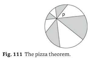
In Acheson's The Wonder Book of Geometry, I came across the "pizza theorem."

The basic form of the problem says to take any point within a disk, and construct a grid of chords which all cross at that point. There are two pairs of perpendicular chords, evenly spaced at 45 degrees.

Alternate radial sections are shaded. The result is that the pizza is always evenly divided between light and dark pieces, even though the pieces themselves are oddly shaped.

Here is Acheson's figure.

If the grid coincides with the center of the circle, the theorem is obviously correct. And if the grid moves by sliding along a diagonal of the circle, for example vertically, the result is still correct. That's because the figure has mirror-image symmetry.

After a vertical move to move to the desired final radial position, the grid can be either rotated or moved "horizontally", parallel to a chord but not on a diagonal of the circle. I worked out a geometric proof that this movement does not change the relative areas.

The basic idea is that the areas gained and lost by the movement go like the difference t-s for the two parts of each chord. (Except that the area covered by the vertical chord is fatter by sqrt(2)).

But that difference is closely related to the distance from the center of the chord to the grid center. The sum of those is easily shown to be invariant, because the center of each chord lies on its vertical bisector, which passes through the center of the circle.

I also found on the web a nice geometric proof for invariance under rotation (first answer at the link). I expanded it to make it (hopefully) even clearer (pdf).

I also added a chapter to my geometry book (38 MB). There are shorter versions elsewhere that I linked previously, but they are now outdated.

Monday, February 28, 2022

Comments

I've had to turn comments off for the blog. Nothing but spam anymore. The intrepid reader will be able to find me. Hint: +"9" and I use gmail.

Wednesday, September 15, 2021

Sum of angles: Ptolemy

 The "sum of angles" theorems are incredibly useful in calculus.  These are formulas for the sine (or cosine) of the sum (or difference) of two angles.  There are a number of derivations, of which my favorite is a proof-without-words (here).

Recently, I got interested in Ptolemy's theorem, which is illustrated in this graphic:


There are proofs based on similar triangles (a bit complicated), and one based on areas with a wonderful trick in the middle.  Another terrific proof-without-words for that is here.

It turns out that there are easy proofs for the trigonometric theorems starting from Ptolemy's theorem, and I want to look at them here.  The first one is for sin s+t:

The proof depends on the following details.  First, the black line in the middle is a diameter of the circle, scaled to have length 1.  As a result, the two triangles are right triangles, justifying the labels on the sides.  Ptolemy says to multiply two pairs of opposite sides and add them.

In addition, the dotted line is the chord of the sum of the two angles, and its length is:  2R sin s+t = L.  But 2R is scaled to be 1, so finally we have the formula for the sine of s+t.  It basically writes itself.

The second one is for the difference.  This is extra, since the easiest way to get from the sum to the difference is to use the fact that cosine is an even function and sine is odd:  sin(x) = -sin(-x).

If you're trying to set this up yourself, a big clue is that since the formula has a minus sign in it (sin s cos t minus sin t cos s), the sin s-t term is going to be one of the sides, and naturally, it is the side opposite the diameter.

As for the cosine formulas, there is yet another trick.  We will still have that the dotted line is going to be the sine of some angle θ, but it is also the cosine of the angle that is complementary to θ!  And again, cosine s+t is one of the sides.


The last one isn't quite as pretty (I don't know if there are others, I came up with this one myself).  The hard part is writing an expression for the angle marked with the black dot, but its complement is just s-t.


Wednesday, August 25, 2021

Calculating continued fractions

 I've been playing with continued fractions.  The golden ratio is one of the simplest examples.


Substituting the whole right-hand side for the denominator on the right:

And here is sqrt(3) for another.  I find the square root symbol to be a bit of a distraction, so I substituted x for sqrt(3).

The standard notation for this is [1;(1,2)].  Here is the derivation for this example:


At this point, the trick is to add and subtract 1 in the denominator on the right-hand side  

But (x - 1)/2 = 1/(x + 1), and after another round of add and subtract we have

We are done because x - 1 appears on both sides.

Then to evaluate it we must chop off the continuation somewhere.  For this example, there are two different chains of rational approximations to sqrt(3).  Here is one


I think I finally understand how the derivation works.  I've done a number of examples with as many as 8 terms in the continued part.  This resource was very helpful, since it has the correct answers.

I also wrote a simple Python script to evaluate a continued fraction based on the coefficients, which does the somewhat tedious calculations.

I wrote this up as a pdf on GitHub, and the script is a gist here.

And finally, just note that the existence of a continued fraction that continues forever is a proof of irrationality.  All of the integers that are not perfect squares are irrational, and they all have continued fraction representations.

[Sorry for the large image sizes.  They are screenshots from my pdf, which blogger insists on making giant size even when "small".  I know, I know, MathJax, but ... ].

Friday, July 16, 2021

Pentagons, again

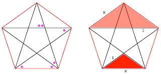
 It's been some years, but I took another look at pentagons.  It is fun to see the connection between φ,  the "golden ratio", and the internal triangles in a pentagon.

First of all. the figure has five-fold rotational symmetry.

The marked angles in the panel on the left are equal by the isosceles triangle theorem, so the angles on either side of the central angle at each vertex are equal.  

Then we do some addition:  3 black + 2 magenta = 180 = 4 magenta + 1 black.  We conclude that black = mageneta.  So the vertex angle is divided into 3 equal parts.


The small triangle at the top is isosceles, because the triangles on either side are congruent to each other (by rotational symmetry, or ASA), so both sides are equal. Now, we see that the horizontal chord is parallel to the bottom side, by alternate interior angles.  We have a bunch of rhombi!

There are two types of similar triangles:  one tall and skinny, the other short and squat.

In the right-hand panel, a triangle of the second type is shown in light red.  It has equal sides of length x and a base of length x + 1.  The red one has sides of length 1 and a base of length x.  We form the equal ratios:  (x+1) /x = x.

One can also use the tall skinny triangles.

This allows the base to have length 1.  Then, the sides of the tall skinny triangle in the middle are x.  The small, tall skinny triangle at the top has sides x - 1 and base x - 2(x - 1) so the ratios of similar triangles are x = (x - 1)/(-x + 2), which simplifies to the same expression as before.


The apex angle of a tall skinny triangle is equal to 1/3 of the interior angle of the pentagon, which is 108/3 = 36.

We will find an expression for the sine of 36°, and this will give us another way to calculate the side length for the pentagon in terms of the chords.

We start by working with 18°, because 90/18 = 5 exactly.  The trick is that (using θ for 18°):  5θ = 90° so 2θ = 90 - 3θ.  Taking the sine of both sides and then converting to the complementary angle on the right, we have sin 2θ = cos 3θ.

One can also use de Moivre's formula and take the real part.

[Since φ - 1 = 1/φ, the above result can be written more simply, but it makes the calculation below more complicated].


There is something else.  If one draws the central angles of the pentagon, then the triangle containing a central angle of 72° and a base of one side length has a half angle of 36°.

So one-half the side length is the sine of 36°, which we found above.  The circle containing the five vertices for a pentagon of side length 1, has a radius of r = 1/2 sin36° = 1/sqrt(3 - φ).

The pdf of the write-up is here (Latex one level down).